Neural Network Architecture for Detecting Traffic Signs
Design a convolutional neural network to classify traffic signs. Starting with the LeNet architecture and improving its generalization and accuracy.

The goal of this project is to design a convolutional neural network to classify traffic signs. Other architectures are explored such as GoogLeNet. I started with the LeNet architecture and then added inception modules and dropout.
The goals/steps of this project are the following:
- Load the data set (Download Here)
- Explore, summarize and visualize the data samples
- Design, train and test the model architecture
- Use the model to make predictions on new images
- Analyze the softmax probabilities of the new images
Training, Validation and Testing Data Size
I used numpy to calculate summary statistics of the traffic signs data set:
- Size of training set: 34799
- Size of the validation set: 4410
- Size of test set: 12630
- Shape of a traffic sign image: 32x32 (RGB)
- The number of unique classes/labels: 43
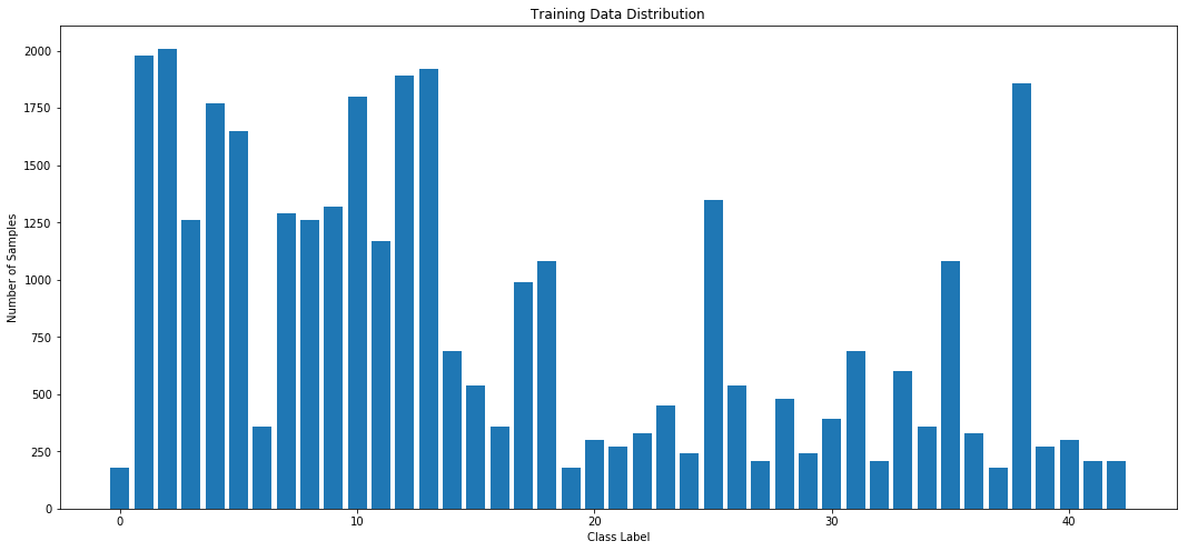
Distribution of Training Data
Here is an exploratory visualization of the data set. The bar chart shows the distribution of training samples by class label.
Convolutional Neural Network (CNN) Model Architecture
Preprocessing Data Sets
The first step is grayscaling the images to increase performance during training.
However, there may be some cases where the color can be significant, although I
haven't explored this.
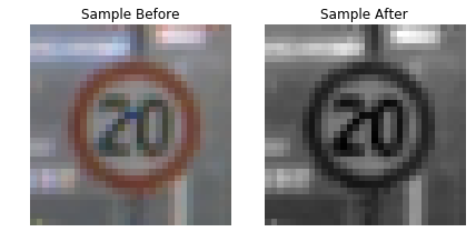
The image is also normalized to improve training performance, making the grayscale pixel numerical values between 0.1-0.9 instead of the range from 0-255.
Here is an example of a traffic sign image before and after grayscaling and normalization.
Model Architecture
My final model consisted of the following layers. I started with the LeNet architecture and then followed the paper on GoogLeNet by adding inception modules, average pooling followed by 2 fully connected layers with dropout in between both.
| Layer | Description |
|---|---|
| Input | 32x32x3 RGB image |
| Preprocessing | 32x32x1 Grayscale normalized image |
| Convolution 5x5 | 1x1 stride, valid padding, outputs 28x28x6 |
| RELU 1 | Activation |
| Convolution 5x5 | 1x1 stride, valid padding, outputs 24x24x16 |
| RELU 2 | Activation |
| Average pooling 1 | 2x2 stride, outputs 12x12x16 |
| Inception Module 1 | outputs 12x12x256 |
| Average pooling 2 | 2x2 stride, outputs 6x6x256 |
| Inception Module 2 | outputs 6x6x512 |
| Average pooling 3 | 2x2 stride, same padding, outputs 6x6x512 |
| Dropout 1 | Flatten the output and dropout 50% layer |
| Fully connected 1 | Outputs 9216x512 |
| Dropout 2 | Dropout 50% layer |
| Fully connected 2 | Outputs 512x43 |
| Softmax | Softmax probabilities |
Training the Model
- Preprocessed the images
- One hot encoded the labels
- Trained using Adam optimizer
- Batch size: 128 images
- Learning rate: 0.001
- Variables initialize with truncated normal distributions
- Hyperparameters, mu = 0, sigma = 0.1, dropout = 0.5
- Trained for 20 epochs
Training was carried out on an AWS g2.2xlarge GPU instance. Each epoch was completed in around 24s, total training time of about 6-8 minutes.
Designing the Model
Final model results:
- Validation set accuracy: 0.97
- Test set accuracy: 0.95
The approach started with a review of LeNet and GoogLeNet architectures and those were used as a starting point to decide how to order and how many inception modules, pooling convolution and dropout layers to use.
- First started with LeNet and with minor tweaks, achieved an accuracy of about 0.89
- Reduced and switched max pooling to average pooling to get to 0.90
- Added an inception module after the first two convolutions to get to 0.90-0.93
- At this point, there were very deep inception modules (referencing GoogLeNet) and 4 fully connected layers and the model appeared to be overfitting.
- Reducing the number of fully connected layers to 2 and adding dropout between them made the largest impact and achieved around 0.97 accuracy.
Once I noticed the accuracy starting high and surpassing the minimum 0.93, I tweaked the layers by trial and error but my approach was to try and keep as much information flowing through the model while balancing the dimensional reduction. This led me to have 2 convolution layers with small patch sizes, average pooling with small patch size and do more severe reductions with the inception modules.
Test a Model on New Images
Here are some other German traffic signs that I found on the web. The signs are
generally easy to identify, I chose a few that are at angles and one that had a
"1" spray painted onto a 30km/h sign.
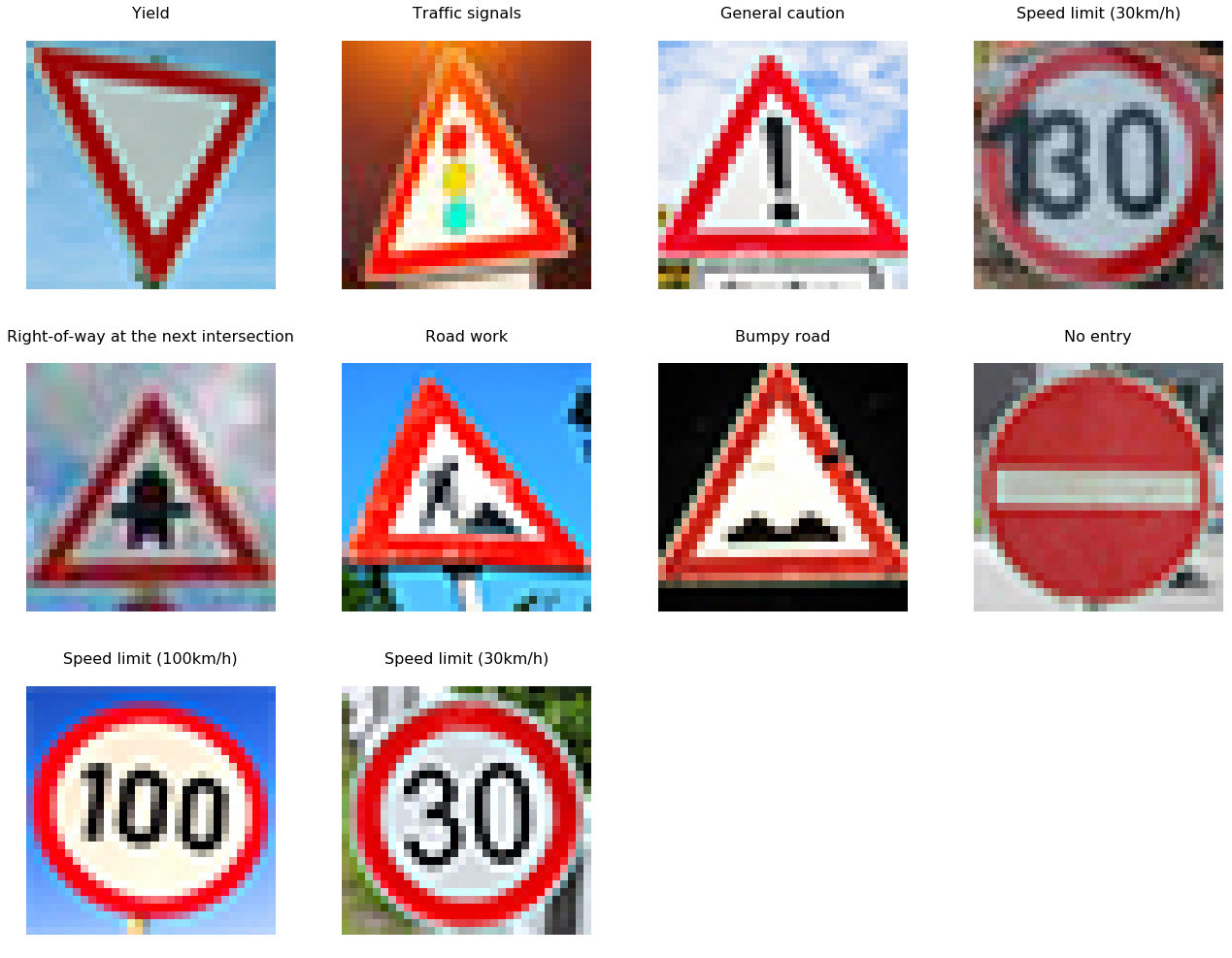
New Image Test Results
Here are the results of the predictions on the new traffic signs:
| Image | Prediction |
|---|---|
| Yield | Yield |
| Traffic Signals | Traffic Signals |
| General Caution | General Caution |
| Speed Limit 30 | Speed Limit 30 |
| Right of Way | Right of Way |
| Road Work | Road Work |
| Bumpy Road | Bicycles Crossing |
| No Entry | No Entry |
| Speed Limit 100 | Roundabout Mandatory |
| Speed Limit 30 (spray painted) | Speed Limit 30 |
The model was able to correctly guess 8 of the 10 traffic signs, which gives an accuracy of 80%. I was impressed that the spray-painted sign still classified correctly even though the clear 100km/h sign was wrong.
The bicycles crossing and bumpy road signs do look very similar at low resolution, so I can understand that wrong prediction.
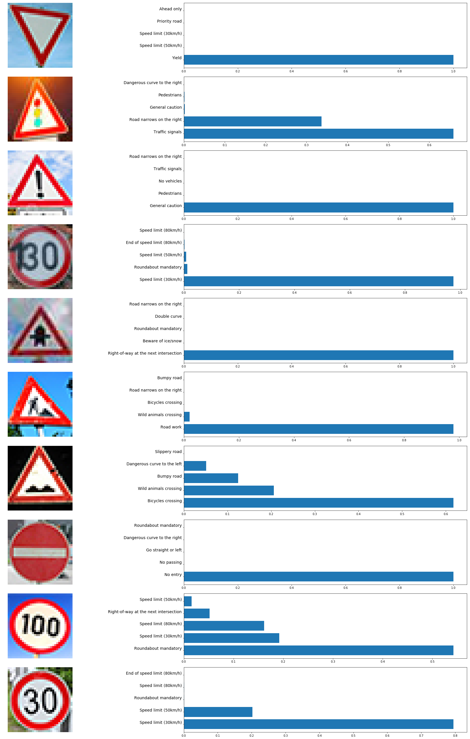
Model Certainty
The following shows the top 5 softmax probabilities for each sign.
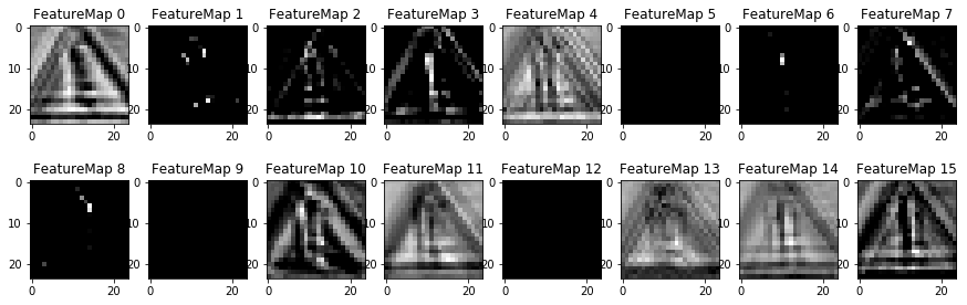
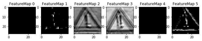
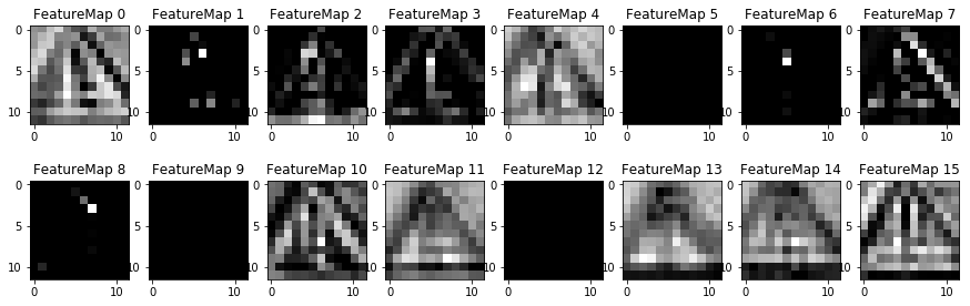
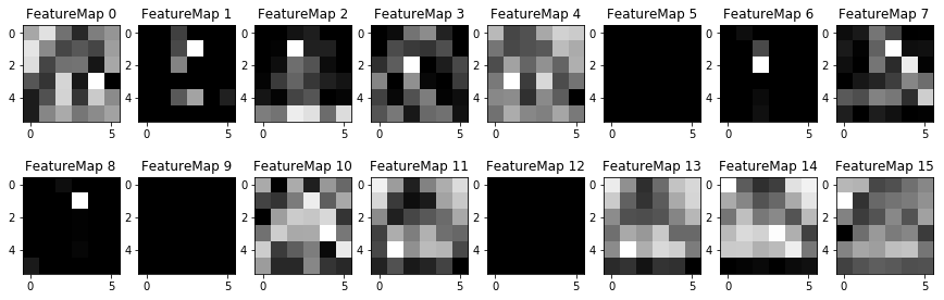
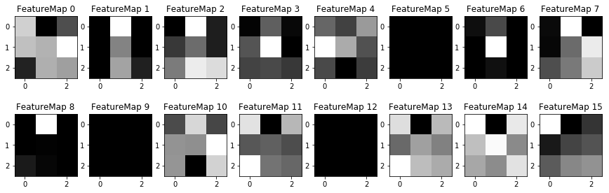
Visualizing the Model Layers
It's interesting to see the layers of the network as it progresses. The convolution layers look the most interesting, while the average pooling layers start to look overly simplified. However, the average pooling images only show one layer in a very deep set.

Conclusions and Discussion
Having LeNet and GoogLeNet as starting points was very helpful. There are still many areas for improvement by tweaking variables, moving/adding/removing layers and augmenting the data set. I noticed that when applying the GoogLeNet architecture directly to this data set, the training time was very high and accuracy plateaued quickly which could indicate over/underfitting. But in this case, I believe there were too many parameters, I found better performance by reducing the depth of the inception layers and adding dropout.
Check out the GitHub repo for the code and Jupyter Notebook.