Simple State Space Model of a Pendulum

This is the first post of a series that will build on simple pendulum dynamics to investigate different control laws and how model uncertainty affects the linear model approximation.

Pendulum diagram and Free Body Diagram

Pendulum Model

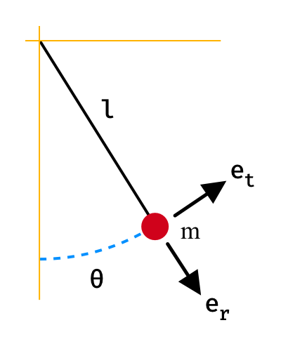
We will start by deriving the equations of motion for the simple pendulum shown below. The mass $m$ is suspended by a massless rod of length $l$. The angle $\theta$ is measured from the downward vertical with positive counter clockwise direction. The vectors $e_r$ and $e_t$ are the radial and tangential unit vectors respectively.

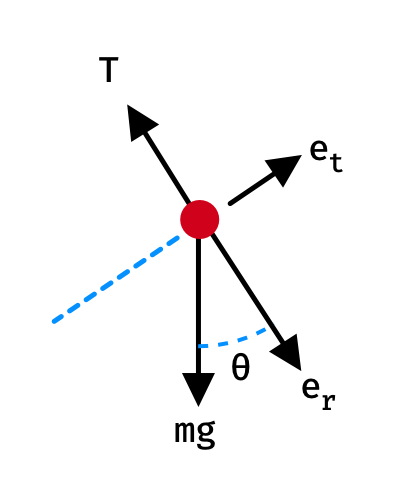
The first step is to draw a free body diagram showing all the forces acting on the mass. Using Newton’s Second Law to write the equations of motion for the mass (in radial coordinates).

$$\begin{alignedat}{1} T - mg\cos\theta &= m\ddot{r}_{e_r} \\ -mg\sin\theta &= m\ddot{r}_{e_t} \end{alignedat}$$

Assume the length of the rod is constant, then $\dot{r}$ and $\ddot{r}$ in the $e_r$ direction are both zero. Now we must find the tangential component $\ddot{r}_{e_t}$. To do this, we write position as a vector from the origin to the mass and take derivatives as follows:

$$\begin{alignedat}{1} r &= l{e_r} + l\theta{e_t} \\ \dot{r} &= l\dot{\theta}{e_t} \\ \ddot{r} &= l\ddot{\theta}{e_t} \end{alignedat}$$

Now we can substitute this into our dynamics equations and get the following:

$$\begin{alignedat}{1} mg\cos\theta &= T \\ -mg\sin\theta &= ml\ddot{\theta} \\ \end{alignedat}$$

Simplifying the second equation and rearranging gives us the nonlinear ODE of the mass:

$$\begin{alignedat}{1} \ddot{\theta} = -\frac{g}{l}\sin\theta \end{alignedat}$$

State Space Form

To get the above equation into state space form, start by introducing a change of variable that will reduce the order of the ODE:

$$\begin{alignedat}{1} x_1 &= \theta \\ x_2 &= \dot{\theta} \end{alignedat}$$

Then take derivatives of these two substitutions and it follows:

$$\begin{alignedat}{1} \dot{x_1} = \dot{\theta} &= x_2 \\ \dot{x_2} = \ddot{\theta} &= -\frac{g}{l}\sin{x_1} \end{alignedat}$$

Jacobian

Calculate the Jacobian by first taking partial derivatives of the equations above with respect to each variable: $x_1$ and $x_2$.

$$\begin{alignedat}{1} J &= \frac{\partial\boldsymbol{f}}{\partial{\boldsymbol{x}}}\Big|_{\tilde{x}} \\ &=\tfrac{\partial}{\partial{x}} \begin{bmatrix} x_2 \\ -\frac{g}{l}\sin{x_1} \end{bmatrix} \\ &= \begin{bmatrix} 0 & 1 \\ -\frac{g}{l}\cos{x_1} & 0 \end{bmatrix} \Big|_{\tilde{x}} \\ \end{alignedat}$$

The state space model can be created by evaluating the matrix of partial derivatives at the nominal trajectory $\tilde{x} = (\pi, 0)$, the result is the Jacobian.

$$A = \frac{\partial}{\partial{x}}f(\tilde{x}) = \begin{bmatrix} 0 & 1 \\ -\frac{g}{l} & 0 \end{bmatrix}$$

State Space Form

The final linear model can now be represented as follows:

$$\dot{x} = \begin{bmatrix} 0 & 1 \\ -p & 0 \end{bmatrix} x$$ $$where \quad p = \frac{g}{l}$$

Stability

Looking at the matrix $A$, we see it is full rank and controllable, however there is no control signal present in this example. We can check the stability of the nominal trajectory by looking at the eigenvalues of $A$ by solving for the roots of $det(A - I\lambda)$. Solving for $\lambda$ results in $\lambda = \pm\sqrt{p}$, with one positive real root indicating the system is unstable around $\tilde{x} = (\pi, 0)$.

As a quick example, picking the equilibrium point of $(0, 0)$ (downward resting position) results in eigenvalues of $\lambda = \pm{i}\sqrt{p}$ with no real part. Given this model, a perturbation of the pendulum from its downward resting point will continue to oscillate indefinitely.