
Simple Inverted Pendulum: Linear State Feedback Control
We will start with that linear model and introduce a control $u$ proportional to the torque at the attachment point.
Referring to the post on the State Space Model of a Pendulum, we will start with that linear model and introduce a control $u$ proportional to the torque at the attachment point.
We can then simulate state feedback control and observe the response of the system. This post is limited to simulation on the linearized dynamics, so no surprise, we'll see asymptotic stabilization around the nominal trajectory.
With this model and uncertain parameter $p$, we will design a state feedback control law that stabilizes the inverted position $\tilde{x} = [\pi, 0]$ and look at the system response around that nominal trajectory and the effects of $p$.
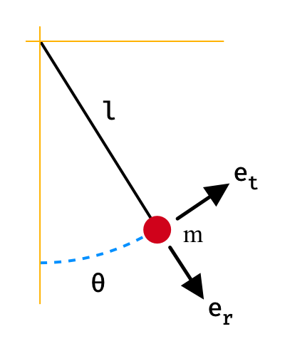
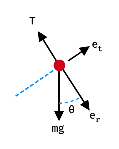
\begin{equation} \begin{alignedat}{1} \dot{x}_{1} &= x_{2} \\ \dot{x}_{2} &= -p \sin{x_{1}} + u \end{alignedat} \end{equation}Where $x_{1}$ is the angle of the pendulum measured from the downward vertical, $x_{2}$ is the angular rate of the pendulum and $p$ is an uncertain parameter that can vary $p_{min} \le p \le p_{max}$.
The first step in designing the linear state feedback control law is to look at the linearized dynamics around the nominal trajectory. Put the above nonlinear equations into state-space form by defining $f(x,u)$, and take an output to be the angle of the pendulum as $h(x,u)$.
\begin{equation} \begin{alignedat}{1} f(x,u) = \begin{bmatrix} x_2 \\ -p\sin{x_1} + u \end{bmatrix}, h(x,u) = x_1 \end{alignedat} \end{equation}Now differentiate each equation with respect to each variable and evaluate the nominal trajectories.
\begin{equation} \begin{alignedat}{1} A = \tfrac{\partial}{\partial{x}}f(x,u)\Big|_{\tilde{x}} &= \begin{bmatrix} 0 & 1 \\ -p & 0 \end{bmatrix} \\ B = \tfrac{\partial}{\partial{u}}f(x,u)\Big|_{\tilde{x}} &= \begin{bmatrix} 0 \\ 1 \end{bmatrix} \\ C = \tfrac{\partial}{\partial{x}}h(x,u)\Big|_{\tilde{x}} &= \begin{bmatrix} 1 & 0 \end{bmatrix} \\ D = \tfrac{\partial}{\partial{u}}h(x,u)\Big|_{\tilde{x}} &= \begin{bmatrix} 0 \end{bmatrix} \end{alignedat} \end{equation}Now we define the deviation of the state from the nominal trajectory as:
\begin{equation} \begin{alignedat}{1} x_{\delta} &= x - \tilde{x} \\ u_{\delta} &= Kx_\delta \end{alignedat} \end{equation}Substituting into the state space model we have the following open-loop dynamics:
\begin{equation} \begin{alignedat}{1} \dot{x_\delta} &= Ax_\delta + Bu_\delta \\ y_\delta &= Cx_\delta \end{alignedat} \end{equation}With state feedback control of $u_\delta=-Kx_\delta$, we get the following closed-loop dynamics:
\begin{equation} \begin{alignedat}{1} \dot{x_\delta} &= (A - BK)x_\delta \\ y_\delta &= Cx_\delta \end{alignedat} \end{equation}Simulations shows the response under increasing initial conditions on the angle and angular rate.
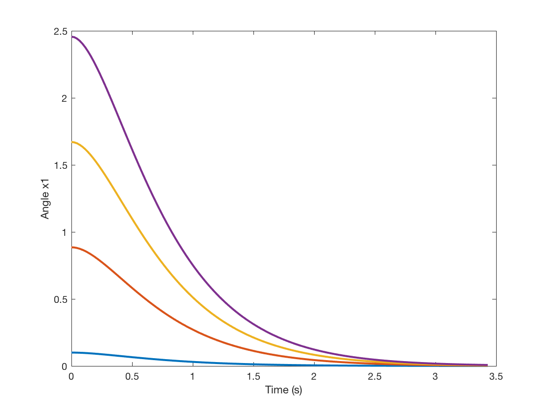
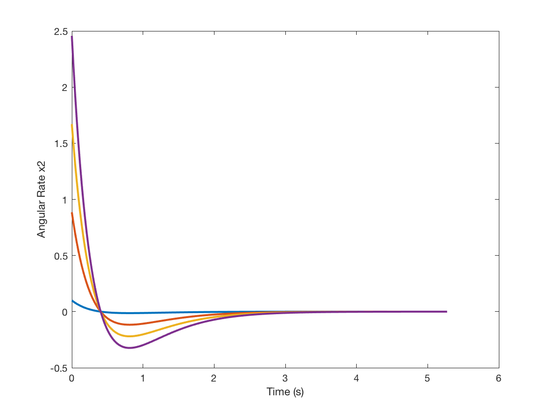
Notice that even with large angle and angular offsets, the system is still stabilized (asymptotically). No surprise though, this simulating a linear model and this is the expected response. In the next post we will simulate this control law but using the nonlinear dynamics and observe the differences.
% Jacobian Linearization of simple inverted pendulum
clear; close all; clc;

% Define some symbols
syms x1 x2 p x1 u

% Nonlinear dynamics
% x1 is angle of pendulum from downward vertical
% x2 is angular rate of pendulum
x1dot = x2;
x2dot = -p*sin(x1) + u;

% x and u input vectors for Jacobian function
Vx = [x1;x2];
Vu = [u];

f = [x1dot; x2dot];
A = jacobian(f, Vx);
B = jacobian(f, Vu);
C = [1 0];
D = [0];

% Evaluate the Jacobian matrices at equilibrium points and
% define the unknown parameter p
x1 = pi;
x2 = 0;
p = 1;

A = eval(A);
B = eval(B);

% Define where the poles should be
poles = [-2; -3];

% Calculate K by placing the poles of (A-BK)
K = place(A, B, poles);

% Create the state space model
sys = ss(A-B*K, B, C, D);

figure(3);

% Increase the initial angle
for m = 0.1:pi/4:pi
  x0 = [m; 0];
  [~,t,states] = initial(sys,x0);
  x1 = states(:,1);
  x2 = states(:,2);

  plot(t, x1, 'LineWidth', 2);

  xlabel('Time (s)');
  ylabel('Angle x1');

  hold on;
end

figure(4);

% Increase the initial angular rate
for m = 0.1:pi/4:pi
  x0 = [0; m];
  [~,t,states] = initial(sys,x0);
  x1 = states(:,1);
  x2 = states(:,2);

  plot(t, x2, 'LineWidth', 2);

  xlabel('Time (s)');
  ylabel('Angular Rate x2');

  hold on;
end
The MATLAB follows the same steps outlined here by calculating the Jacobian, evaluating at the nominal trajectory and forming the closed loop dynamics. We can use MATLAB's $place$ command to obtains the value of $K$ that places the poles of $(A - BK)$ at desired locations. With closed-loop dynamics defined, MATLAB's $ss$ function provides a state-space model that can be used to observe system responses.